1.- Network Structure: Construction and Metrics
1.1- What is a network?
A network (or graph in mathematics) is a set of elements with specific characteristic relationships between them. We call the elements vertices (or nodes) and the relations between them edges (or links). In the picture below we can see a network composed of 8 nodes and 10 links between them.
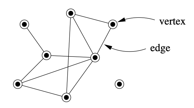
There are a couple of things to be noted about this network, which we will revisit later on. The links between the nodes do not have an apparent directionality, making this an undirected graph. On the other hand, when the direction between link is relevant, such as for example in a predator-prey interaction, where it is convenient to represent the fact that the flow of biomass runs from prey to predator, the links might be represented as arrows. Networks represented in this way are called directed graphs.
Secondly, one of the nodes is isolated. Can you guess which one it is?
You might have started noticing that depending on the types of links, and their placement between nodes within the network, there are a few categories under which we can classify networks according to their features. Two categories are relevant for this course:
1.- Networks can be either directed or undirected as we saw before.
2.- Depending on the constraints of connectivity between groups of nodes, networks can be classified as either unipartite where all nodes could in principle be connected to any other node, or bipartite, where two different groups of nodes exist in which links between nodes in different groups occur but links between nodes within the same group do not.
We will encounter both unipartite and bipartite networks along the way. Watch out!
Many systems both natural and man-made, can be thought of as networks. From the network of airports around to world and the air routes connecting them, to the World Wide Web and the links between web pages, or social networks of friendships (both real and digital), all the way down to microscopic entities such as gene and metabolic networks, these systems can be represented and, perhaps more importantly, analysed as networks.

The field of mathematics has been studying networks for decades. The
mathematics subfield of Graph Theory has
developed extensive frameworks to analyse and manipulate mathematical
objects known as graphs. Graphs, as networks, are simply
collections of nodes and links between them. So, we can represent
networks as graphs and take advantage of the mathematical framework of
Graph Theory to study them.
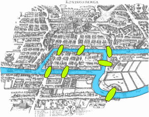
The mathematical study of graphs (or networks) arguably started in 1735 when the celebrated mathematician Leonhard Euler, yes!, the same one who introduced the e as the base of the natural logarithm, developed what is considered the first theorem of graph theory to solve the problem known as the Seven bridges of Königsberg.
Ever since then, the application of graph theory has percolated the sciences. It started back in the 1930s when tools for the analysis of networks were applied to the social sciences to develop a better understanding of social relationships among humans.
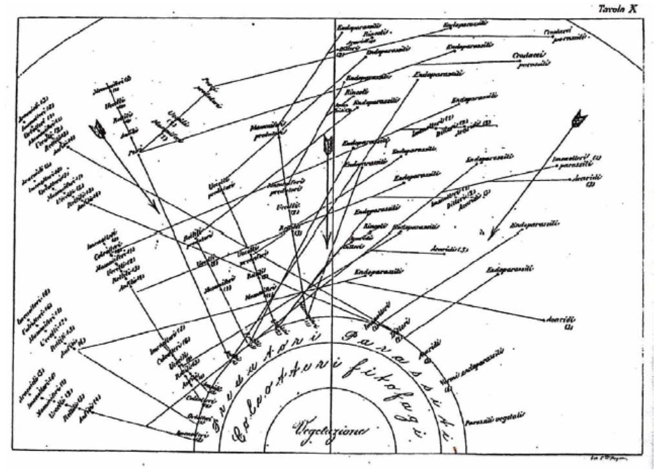
In ecology, even though network representations of natural communities can be traced back to the 1880’s in the work by Lorenzo Camerano, the quantitative analysis of networks and their properties, as well as their mathematical modelling, started much more recently, around the 1960’s - 70’s.
In the following sections we will learn how to analyse networks.
Our focus will be networks of ecological interactions between species
sharing the same ecological community. In very diverse systems these can
be up to 1,000’s of species. As such, many of the quantities we will be
learning about are mostly relevant to quantify
biodiversity and can be seen as a natural extension to
the classical analysis performed in community ecology.
Nonetheless, the underlying principles of network construction and
analysis can be applied to any networked system, including those
mentioned above.
1.2- Network formats: edgelists and adjacency matrices
To be able to manipulate and analyse networks in an automated way, we need to represent them in a way that is understandable by a computer. Several computer readable formats exist to store the description and information contained in a network. The most commonly used in ecology (and other disciplines) are: (i) adjacency matrices, and (ii) edgelists.
Adjancecy matrices, one of the most common ways of representing networks in mathematics, are matrices in which columns and rows represent the nodes (species) in the network, and a link (interaction) between them is represented as a 1, while the absence of a link is represented as a 0.
In a foodweb, for example, as we saw previously, links are directed from prey to predator. In the adjacency matrix, the rows represent prey species and the columns represent predators. Thus, an interaction aij runs from prey i to predator j.
Adjacency matrices are good for representing unipartite networks because in principle there could be a connection between any two nodes. In bipartite networks on the other hand, as we saw before, we know in advance that some links cannot occur (i.e. those between nodes within the same groups). As such all nodes do not have to be represented in each dimension of the matrix (rows and columns) but only in one of them. This gives rise to a slightly different format from an adjacency matrix, but where the meaning of the elements in the matrix is still the same. These are incidence matrices. In and incidence matrix one set of nodes is represented by the rows and the other one by the columns. Links thus connect nodes in the the rows with nodes in the columns. This makes these matrices non-square.
An added virtue of the incidence matrix format is that it saves us a lot of space in the computer (and in our notebooks if we were using pen and paper!). Can you figure out why?
Can you think of a few examples of ecological networks that can be represented as bipartite and thus as incidence matrices?
That’s right! Mutualistic networks (e.g. plant-pollinator) are bipartite. As such, they can be represented as incidence matrices, where hosts are usually shown in rows and their mutualistic partners are shown in columns.
Edge lists, on the other hand, are lists of pairs of identifiers (usually integers) that denote links (or ecological interactions) from the first item in pair to the second. For example, a network specified by the following edge list:
1 2
2 3
1 3
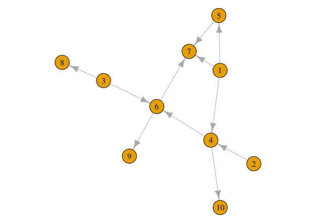
is one with three nodes: V = {1,2,3}, and three links: one from basal prey 1 to primary consumer 2, another one from prey (primary consumer) 2 to top predator 3, and finally, an interaction between the basal resource and the top predator (E = {(1,2), (2,3), (1,3)}). This makes the top predator an omnivorous species. A representation of this network is shown below:
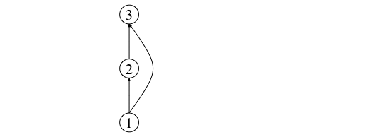
This network can be represented as an adjacency matrix thus:

More sophisticated ways of representing and storing networks exist, such as for example the GraphML format, in which additional information about the network, the nodes, and the links can be included in the description. During these lectures, we will use a mixture of different formats to represent networks in text files (e.g. edge lists, adjacency matrices, etc).
Throughout the course we will use a few examples of real ecological networks taken publicly available databases such as the well-known food web from the Benguela upwelling marine system off the Western coast of Africa:

Image taken from Yodzis, P (1998) Local trophodynamics and the interaction of marine mammals and fisheries in the Benguela ecosystem. Journal of Animal Ecology. 67, 635-658.
This, and other ecological networks datasets, are available from the Global Food Web Database.
The code below will enable you to download the edgelist file and use
it to create an adjacency matrix representation of the network. Two
representations of the network then remain available: the Edgelist
representation (benguela.EL) and the Adjacency Matrix
representation (benguela.AM).
library(RCurl)
x <- getURL("https://raw.githubusercontent.com/mlurgi/networks_for_r/master/datasets/benguela.edgelist")
benguela.EL <- read.table(text = x)
benguela.EL <- as.matrix(benguela.EL)
# Create an adjacency matrix called benguela.AM, containing only zeros
benguela.AM <- matrix(0, max(benguela.EL), max(benguela.EL))
# Introduce ones to the matrix to represent interactions between species
benguela.AM[benguela.EL] <- 11.3- Species and interactions as vertices and links
In abstract representations of ecological communities as networks, nodes represent species and links amongst them denote ecological interactions happening between the represented species.
Adjacency matrices are matrix representations of networks where elements of the matrix denote the presence of a link (i.e. interaction) between the species represented by the row and the species represented by the column. Thus, to represent a food web composed of S species as a matrix we need a SxS matrix in order to be able to represent all possible interaction between the S species. The number of species in the network can be calculated thus as the number of rows or the number of columns.
Using the Benguela food web adjacency matrix
benguela.AM, you can calculate the number of species.
In an adjacency matrix, all species are represented by columns and
rows. Counting the number of columns or rows in the adjacency matrix
will let you obtain the number of species in the food web. In R, you can
use the dim function to look at the matrix
dimensions.
# species richness
S <- dim(benguela.AM)[1]Similarly, since interactions are represented as ones in the matrix,
if you sum all the values in the matrix, you will get the
number of interactions.
# number of links
L <- sum(benguela.AM)1.4- Interactions in bipartite networks
Food webs, like that for the Benguela ecosystem studied above, are network representation of who eats whom relationships in an ecological community. As such, there are no distinct subset of species among which interactions are not possible. This is why adjacency matrices for representing food webs contain the total number of species as rows and also as columns. In theory, any interaction is possible.
Other types of ecological networks, however, like for example, plant-animal mutualistic networks (like the figure below) or host-parasite interaction networks, exhibit a bipartite structure. In this type of networks, species can be classified into two distinct groups where interactions do not occur (or are forbidden) among members of the same group. For example, in a plant-animal mutualistic network, plants do not interact with plants and animal mutualists do not interact among them. This feature allows for a more concise matrix representation of bipartite networks.
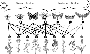
Example of a plant-animal pollinator bipartite network. Image taken from MacGregor, CJ et al. (2015) Pollination by nocturnal Lepidoptera, and the effects of light pollution, a review. Ecological Entomology. 40, 187-198.
As we saw above, the equivalent representation of an adjacency matrix for a bipartite network is called an incidence matrix. In incidence matrices one set of species are represented as rows (e.g. hosts/plants), and the other set of species as columns (e.g. visitors/mutualists). Thus, the way of counting species in an incidence matrix representing a mutualistic (bipartite) network is different from that used to count species in adjacency matrices representing food webs.
For a bipartite ecological network represented by an incidence matrix with size HxV, where H is the number of rows and V is the number of columns, the number of species in the network is equal to H + V.
As an example, we load a matrix representing a bipartite network of interactions between anemones and several species of fish living within them in South-East Asia. This network was taken from Ollerton, J. et al. (2007) Finding NEMO: nestedness engendered by mutualistic organization in anemonefish and their hosts. Proceedings of the Royal Society B. 274, 591-598.
Try and calculate the total number of anemone and fish species in the network. Remember that in a bipartite network, one set of species (in this case, anemones) are represented as columns, while the other set (in this case, fishes) are represented as rows.
library(RCurl)
y <- getURL("https://raw.githubusercontent.com/mlurgi/networks_for_r/master/datasets/anemonefish.txt")
anemonef <- read.table(text = y)
names(anemonef) <- paste("A", 1:10, sep = "")
row.names(anemonef) <- paste("F", 1:26, sep = "")
anemonef <- as.matrix(anemonef)
### The number of fish species in the network is the number of rows
n_fish <- dim(anemonef)[1]
### The number of anemone species is the number of columns
n_anemone <- dim(anemonef)[2]
### So, the total number of species is the sum of these two quantities
S <- n_fish + n_anemone
### Whereas the total number of interactions is still the sum of the matrix
L <- sum(anemonef)1.5- Networks as graphs
As we have seen, edge lists and adjacency matrices are convenient ways in which interaction networks can be represented. However, more flexible formats for representing networks are needed when we want to perform more complex actions on networks, or even just for visualisation purposes.
Several computer programming libraries have been especially developed
to construct and manipulate graphs. These libraries make it easy and
widely accessible to work with and study networks. Amongst the most
popular the NetworkX complex
networks library for Python and
the igraph package for network
analysis, which can be used on several platforms, including R. For the rest of this course we
will be using igraph to create and manipulate ecological
networks.
To install and load igraph on your R workspace run the following commands:
## Install igraph
install.packages("igraph")
## Load igraph into workspace
library(igraph)To start getting familiar with igraph we will start by creating some simple networks.
1.5.1- Weaving networks from scratch
The following instructions will walk you through a simple example in which you will create a small network:
1.- First create a vector called species with the
numbers from 1 to 10
2.- Then create a network by adding the species as
vertices to an empty graph
3.- Create an interaction between species 5 and 7
4.- Create 10 other interactions between any species you want
require(igraph)## Loading required package: igraph##
## Attaching package: 'igraph'## The following objects are masked from 'package:stats':
##
## decompose, spectrum## The following object is masked from 'package:base':
##
## union# Ten species
species <- 1:10
network <- graph.empty() + vertices(species)
# Link between species 5 and 7
network[5,7] <- 11.5.2- Converting matrix to igraph object
If we have an adjacency matrix and we want an igraph object
representing the same network, without the need to create the network
from scratch, igraph offers the functionality of creating graphs from
adjacency matrices. Just use the function
graph.adjacency(A), where A is your adjacency matrix.
Check out the documentation for graph.adjacency,
including additional parameters that you can use to create your network.
Similarly, to create a graph from an edgelist, you can use the
graph_from_edgelistfunction from igraph.
We can convert the network for the Benguela ecosystem, into and igraph object using the following code.
library(RCurl)
x <- getURL("https://raw.githubusercontent.com/mlurgi/networks_for_r/master/datasets/benguela.edgelist")
benguela.EL <- read.table(text = x)
benguela.EL <- as.matrix(benguela.EL)
# Create an adjacency matrix called benguela.AM, containing only zeros
benguela.AM <- matrix(0, max(benguela.EL), max(benguela.EL))

# Introduce ones to the matrix to represent interactions between species
benguela.AM[benguela.EL] <- 1
# Convert Benguela adjacency matrix to an igraph network
benguela.network <- graph.adjacency(benguela.AM)1.5.3- Drawing networks
The network representations we have explored so far are great for manipulating them and calculating properties over them. However, to gain an intuitive idea of what the networks we are analysing look like, or if we want to show them in publications or websites, it is sometimes desirable to draw them as graphs: with dots representing nodes/species and lines connecting them representing links/interactions. In pretty much the same way we saw in the introductory video.
Of course, drawing a network on a whiteboard using coloured pens is easy. Doing that on a computer or writing code in R to do it, might be more of a challenge. Fortunately, libraries such as igraph offer these functionalities. The plot function from the igraph library takes as an input an igraph object and produces a graphical representation of the network.
Let’s try it!
# Plotting your network
plot(network)
If the instructions above worked well you will be able to see something like this:
What about the Benguela ecosystem network…
# Plot the Benguela food web
plot(benguela.network, edge.arrow.size = 0.2)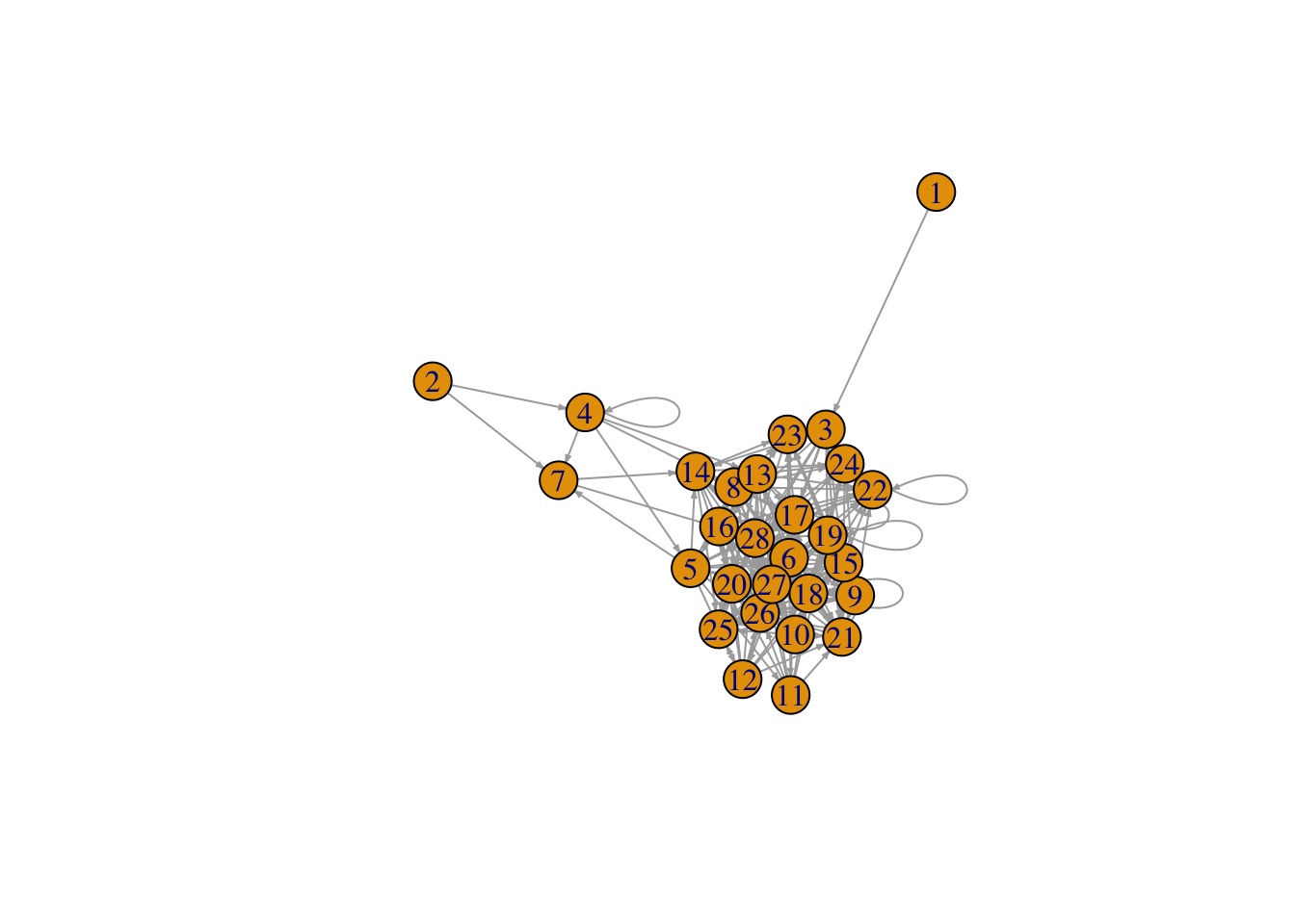
This representation of the Benguela web looks a bit messy. Don’t worry! We will explore ways of making networks more beautiful later on.
1.6- Network Properties
Now that we have an igraph representation of our network(s), we can calculate several of its properties.
1.6.1- Graph connectivity / Food web connectance
If we think of the network we just constructed as a food web, we can calculate the number of species and links (what we did previously on adjacency matrices) thus:
# number of species
S <- vcount(network)

# number of interactions
L <- ecount(network)
The functions vcount and ecount from the
igraph library let you count the number of nodes and links on a graph,
respectively.
Having counted the number of species and links in our newly built
food web, we can start calculating more interesting prorperties such as
connectivity. In food webs connectivity can be quantified as the average
number of interactions per species (L/S, i.e. the mean number of
interactions species in the network have), and Connectance
(L/S2, i.e. the fraction of links present in the network out
of all possible links).
# average number of interactions species
L.S <- L/S

# food web connectance
C <- L/S^2
In the case of the adjacency matrix (A) representation of a food web, we know that it contains all the links in our network represented by 1’s. Hence, the number of links in our network is simply sum(A). Similarly we have also learnt that the number of species (at least for a food web) equals the number of rows (or columns) in the matrix: nrow(A).
Hence, the connectance of our food web represented by matrix A is
calculated as: sum(A)/(nrow(A)2). Try this on your network
above and you should obtain the same quantity we now have in
C. HINT: To obtain the adjacency matrix
representation of an igraph object you can use the
as_adjacency_matrix function.
For the Benguela network we can calculate connectivity properties:
# Calculate connectance
connectance <- ecount(benguela.network) / vcount(benguela.network)^2

# Print connectance va
print(paste0('Connectance of Benguela network =', round(connectance,2)))
## [1] "Connectance of Benguela network =0.25"# Calculate number of links per species
links.per.species <- ecount(benguela.network) / vcount(benguela.network)1.6.2- Connectance in bipartite networks
We have learnt how to calculate the connectance of ecological networks in general: it is simply the fraction of realised links out of the possible ones. Additionally, we have explored methods to quantify connectance in food webs based on the information extracted either from the adjacency matrix or the igraph representation of our networks.
We have also learnt that the way in which bipartite networks are represented in incidence matrices is fundamentally different from the way in which we represent food webs in adjacency matrices. Keeping that in mind, we need to find out ways of finding out what would be: 1.- the correct way of finding out the number of species in a bipartite network from our matrix representation; and 2.- the total possible number of links in a bipartite network (remember that links between species in the same group are ‘forbidden’).
Using the fish-anemone interaction network that we used previously, we can calculate the total number of possible links as the product of the number of species on one side (i.e. fish) times the number of species on the other side (i.e. anemone). This will give us the total number of links if every fish species would be found to interact with each anemone species. Connectance of this network is then simply the total number of links divided by this quantity.
library(RCurl)
y <- getURL("https://raw.githubusercontent.com/seblun/networks_datacamp/master/datasets/anemonefish.txt")
anemonef <- read.table(text = y)
names(anemonef) <- paste("A", 1:10, sep = "")
row.names(anemonef) <- paste("F", 1:26, sep = "")
anemonef <- as.matrix(anemonef)

# Calculate conectance of anemoref
bipartite.connectance <- sum(anemonef) / (dim(anemonef)[1] * dim(anemonef)[2])
Igraph lets us manipulate bipartite networks in a similar way to unipartite ones. We can load the incidence matrix above using the following instruction:
anemonef.network <- graph_from_incidence_matrix(anemonef, directed = TRUE, mode = 'in')And calculate its connectance thus:
# Calculate conectance of anemoref
bipartite.connectance <- ecount(anemonef.network) / (sum(V(anemonef.network)$type) * (vcount(anemonef.network) - sum(V(anemonef.network)$type)) )
As a fun exercise you can try and calculate the average number of links per species in this network!
Aside from the connectivity measures that we learnt in the previous section, more interesting properties can be calculated on ecological networks. In this chapter, we introduce some of these properties and how to calculate them.
1.6.3- Horizontal Diversity : Generality and Vulnerability
Ecological networks are all about species and their interactions. In food webs, these interactions represent consumer-resource relationships, so the set of relationships that a consumer has with its prey is considered the ‘breadth’ of its diet. This diet breadth is a measure of the generality of the consumer species and a mean generality index can be calculated across the network to have an idea of how generalist are species in the network on average. We can calculate generality on the matrix representation of our food webs using the following function:
## Mean generality of species in the network
Generality <- function(M){
  return(sum(colSums(M))/sum((colSums(M)!=0)));
}
Similarly, we can obtain a measure of the average number of consumers that resources on our networks have (i.e. vulnerability) using the following function on our adjacency matrix:
## Mean vulnerability of the species in the network
Vulnerability <- function(M){
  return(sum(rowSums(M))/sum((rowSums(M)!=0)));
}
To be able to compare these quantities across different networks,
they are usually normalised by the average number of links per species
(L/S).
If we are interested in these quantities at the species level, we
simply count their prey or predator numbers or their degree
in the network:
## In-degree or number of prey of all species in the network
InDegree <- function(M){
  return(colSums(M));
}

## Out-degree or number of predators of all species in the network
OutDegree <- function(M){
  return(rowSums(M));
}
Even though these measures are useful to have an idea of the average diet breadth and number of consumers across species in our networks, in many occasions it is desirable to look at the deviation of these properties, since we can have within the same network generalist species such as this guy on the left… … alongside very specialist species, such as this guy on the right…


To assess variability in diet breadth and the degree of vulnerability of species in a food web, metrics such as the standard deviation of normalised generality and vulnerability are useful. These properties can be calculated using the following formulae:
where aij are the i,j values of the adjacency matrix
A representing the food web.
Using R code they can be calculated thus:
## Standard deviation of generality:
SDGenerality <- function(M){
  return(sd(colSums(M) / (sum(M)/dim(M)[1]) ));
}

## Standard deviation of vulnerability:
SDVulnerability <- function(M){
  return(sd(rowSums(M) / (sum(M)/dim(M)[1]) ));
}
1.6.4- Vertical Diversity : Fraction of Species Types
In food webs, we can categorise species according to the role the perform from an ecosystem functioning point of view. Basal resources are species at the base of food chains. They are in charge of converting organic and inorganic compounds into biomass such as, for example, plants or phytoplankton. It is interesting to know the fraction of species in food webs that belong to this category.
## Fraction of basal species
FractionOfBasal <- function(M){
  M_temp <- M;
  diag(M_temp) <- 0;

  b_sps <- sum(which(InDegree(M_temp) == 0) %in% which(OutDegree(M_temp) >= 1));

  return(b_sps / dim(M)[1]);
}
Similarly, knowing the fraction of species belonging to intermediate and top consumer categories can give us information about the degree of predation pressure and top-down regulation expected in the network, and its corresponding community, being analysed.
## Fraction of top predator species
FractionOfTop <- function(M){
  M_temp <- M;
  diag(M_temp) <- 0;

  t_sps <- sum(which(InDegree(M_temp) >= 1) %in% which(OutDegree(M_temp) == 0));

  return(t_sps / dim(M)[1]);
}
## Fraction of intermediate consumer species
FractionOfIntermediate <- function(M){
M_temp <- M;
diag(M_temp) <- 0;
i_sps <- sum(which(InDegree(M_temp) >= 1) %in% which(OutDegree(M_temp) >= 1));
return(i_sps / dim(M)[1]);
}For the Benguela food web we can obtain these properties using the functions defined above.
library(RCurl)
x <- getURL("https://raw.githubusercontent.com/mlurgi/networks_for_r/master/datasets/benguela.edgelist")
benguela.EL <- read.table(text = x)
benguela.EL <- as.matrix(benguela.EL)

# Create an adjacency matrix called benguela.AM, containing only zeros
benguela.AM <- matrix(0, max(benguela.EL), max(benguela.EL))

# Introduce ones to the matrix to represent interactions between species
benguela.AM[benguela.EL] <- 1

gen <- Generality(benguela.AM)
vul <- Vulnerability(benguela.AM)
sdgen <- SDGenerality(benguela.AM)
sdvul <- SDVulnerability(benguela.AM)
B <- FractionOfBasal(benguela.AM)
I <- FractionOfIntermediate(benguela.AM)
T <- FractionOfTop(benguela.AM)
1.6.5- Vertical Complexity : Mean Food Chain Length
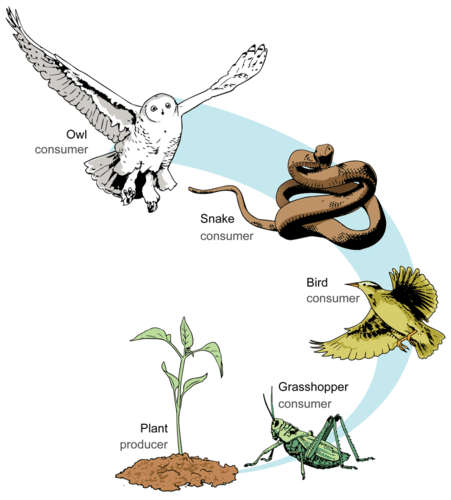
Food chains like those illustrated in the figure above are the exception rather than the norm in nature. Ecological communities are way more complex than this, such as the Benguela food web we saw before. You can imagine a real ecological community as a collection of interconnected food chains. One way to summarise this complexity is to calculate the average length of food chains in the network, i.e. the average number of links from basal resources to top predators or mean food chaing length.
To be able to quantify this, we need to visit all paths in our network running from each basal species to each top predator species. This is a computing intensive task that, for large networks, requires large computational resources (including long execution times). In graph theory and network topology, there is considerable research devoted into how to best count average paths in networks. If you are interested, this is a fascinating area of research and you can play with functions such as distances on igraph to find out more.
In food webs, the paths we are interested in are special because they
all start in basal resources and they all stop at top predators. So, the
way in which we should count those paths is a bit different than what
functions such as distances do. Fortunately, there exist
libraries for food web analysis that can help us calculate metrics and
statistics particularly tailored for food webs. One such a package is cheddar. Cheddar
let’s you calculate all of the food web properties we have seen so far
and many more. We will take advantage of cheddar to calculate mean food
chain length. This will also get you familiar with cheddar and you can
explore many more functionalities offered by the package.
Calculating mean food chain length using cheddar:
MeanFoodChainLength <- function(M){
  require(cheddar)
  M <- t(M)
  node <- 1:dim(M)[1];
  for(n in 1:length(node)){
    node[n] <- paste(node[n],'-');
  }

  pm <- matrix(M, ncol=dim(M)[2], dimnames=list(node, node), byrow=TRUE);

  # We need to convert our adjacency matrix into a Chedday community object.
  # For this, we yse PredationMatrixToLinks()
  community <- Community(nodes=data.frame(node=node), trophic.links=PredationMatrixToLinks(pm), properties=list(title='Community'));

  # We remove cannibalistic links to avoid entering an infinte loop when calculating path lengths
  community <- RemoveCannibalisticLinks(community, title='community');

  chain.stats <- TrophicChainsStats(community)
  ch_lens <- (chain.stats$chain.lengths + 1)

  return(sum(ch_lens)/length(ch_lens));
}
1.6.6- Degree Distributions
Degree distributions constitute a convenient graphical representation of the probabilities of finding a node in a network possessing a certain number of links. This property is important because the shape of the degree distribution of complex networks has been linked to their robustness to random and targeted attacks to their nodes. In particular, networks with degree distributions that follow a power law, which are called scale free networks, are robust against random attacks due to the prevalence of nodes with a small number of links.
Even though the prevalence of truly scale free networks (in the sense of the degree distributions following exactly a power law) has been disputed, networks with degree distributions that display a ‘fat tail’ have been identified in many natural and technological systems from social networks to the internet. Ecological networks are not an exception. This suggests that common underlying principles might be involved in the formation of these networks.
Given its recognised importance and relevance for network persistence we might be interested in obtaining the degree distribution of our ecological networks.
To get the degree distribution of the Benguela network we can follow the instructions below. Since the degree distribution of ecological networks has been suggested to generally follow a truncated power law, we fit that curve to our data.
# degrees of the nodes
degs <- degree(benguela.network, mode='all')

occur = as.vector(table(degs))
occur = occur/sum(occur)
p = occur/sum(occur)
y = rev(cumsum(rev(p)))
x = as.numeric(names(table(degs)))

plot(x, y, log="xy", xlab ='log k', ylab='log Pc(k)', type='p', col='black', pch=16)

box(lwd=1.5)

# and we fit a truncated power law to the data
temp <- data.frame(x,y)
mod1 <- nls(y ~ (x^-a*exp(-x/b)), data = temp, start = list(a = 1, b = 1))

# add fitted curve
lines(temp$x, predict(mod1, list(x = temp$x)), col='red')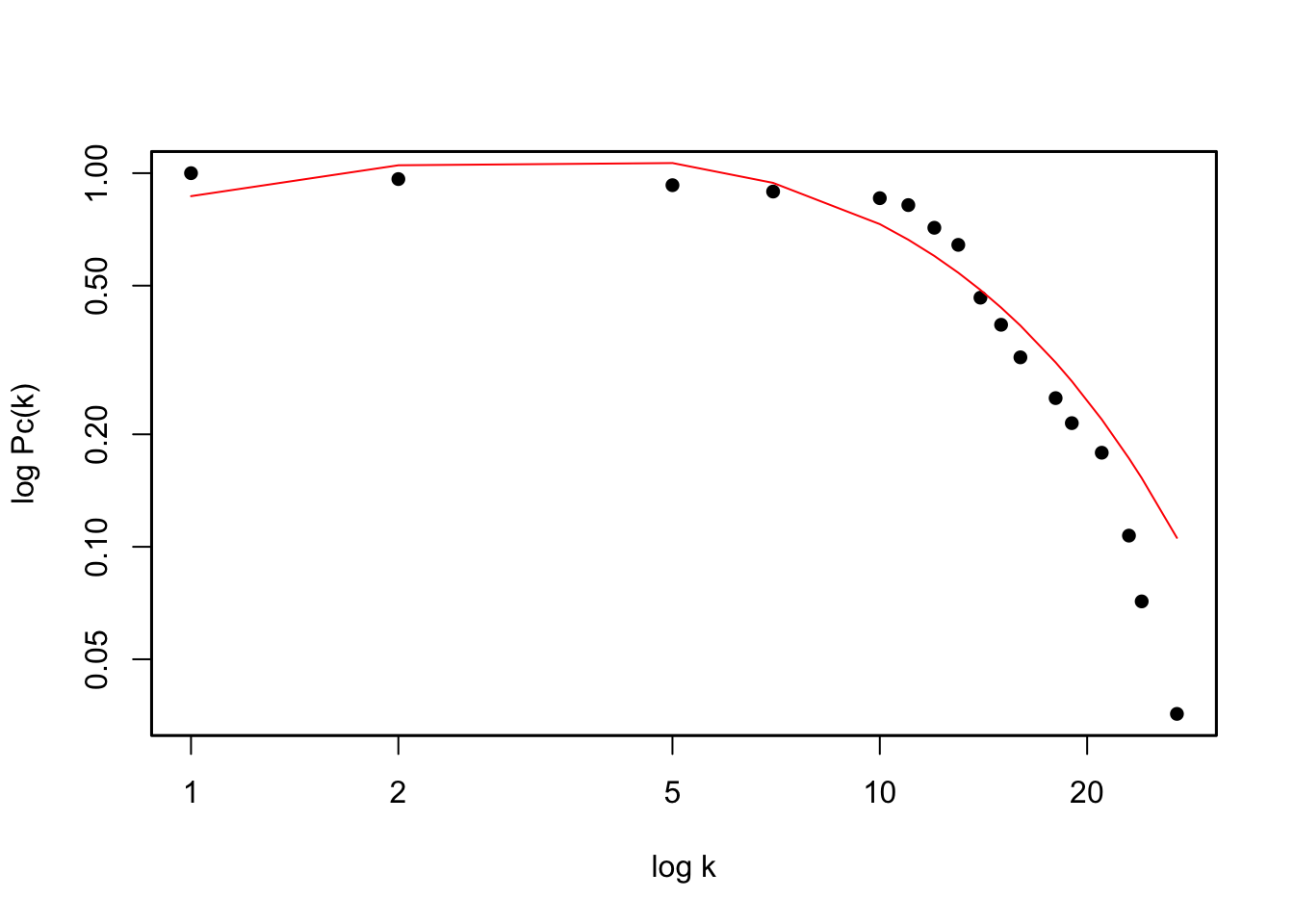
References
Bascompte, J and Jordano P (2007) Plant-Animal Mutualistic Networks: The Architecture of Biodiversity. Annual Review of Ecology, Evolution, and Systematics 38(1), 567-593.
Montoya, J., Pimm, S. & Solé, R. (2006) Ecological networks and their fragility. Nature, 442, 259–264.
Newman, M. E. J. (2003) The Structure and Function of Complex Networks. SIAM Rev., 45(2), 167–256.
Ollerton, J. et al. (2007) Finding NEMO: nestedness engendered by mutualistic organization in anemonefish and their hosts. Proceedings of the Royal Society B, 274, 591-598.